I’ll split the paper explanation into multiple parts. This is the first one:
Circuit tracing is a technique for understanding how large language models (LLMs) work. It involves creating interpretable graph representations that map the model's computational steps using replacement models to reveal the underlying mechanisms of the model's decision-making process. Researchers at Anthropic have developed specialized visualization tools to investigate these attribution graphs.
Circuit tracing involves two essential steps:
- identifying interpretable features or components within the model
- Understanding how these features interact through what are called "circuits."
The low-hanging fruit of approaching Interpretability is to use raw neurons of the model. However, the model neurons don’t represent a single concept, but a mixture of many. This is called polysemanticity, which occurs because models have to represent more concepts than neurons (superposition).
How to build a replacement model?
Cross Layer transcoder: Features read from one layer and write to all subsequent layers.
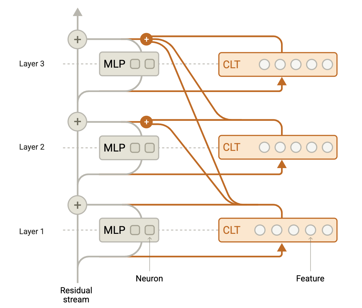
A CLT consists of neurons divided into L layers, the same number as the model. The goal is to reconstruct the model outputs using sparsely active features.
- In the Lth layer, each feature reads from the residual stream at that layer using a linear encoder followed by a nonlinearity.
- An Lth layer feature contributes to reconstructing the MLP outputs in layers L, L+1,…,L using distinct linear decoder weights for each output layer.
- All features in all layers are trained jointly. The MLP output in layer L1 is jointly reconstructed by features from all previous layers.
The replacement model that substitutes the CLT features for the model’s MLP neurons. Each layer’s output is replaced by its reconstruction by all CLTs that write to that layer. Running a forward pass of this replacement model is identical to running the original model with two differences.
-
Before the MLP in layer ℓ: Each layer has a transcoder encoder that transforms the input features into a signal that captures useful info from that layer for later use.
-
After the MLP in layer ℓ: We take the saved signals (from this and earlier layers), run them through decoders that translate them into something layer ℓ can understand. We add up those decoded signals — that becomes the new output for the layers.
What are local replacement models?
The goal is to reproduce the same output as the original model, but there’s a huge gap and errors can compound across layers. To understand the original model, the model should be approximated closely. Therefore a local replacement model which:
- Substitute the CLT for neurons.
- Use the attention patterns and normalization denominators from the the original model’s forward pass
- Adds an error adjustment to the CLT output at each layer equal to the difference between true MLP output and CLT output.
Attribution Graphs

To understand the computations of the local replacement model, we compute a causal graph depicting the computational steps on a prompt. The graphs contain 4 types of nodes:
- The output nodes are constructed for the tokens needed to reach 95% probability mass.
- The intermediate nodes correspond to active cross-layer transcoder features.
- primary input nodes: correspond to embeddings of the prompt tokens
- Additional input nodes: correspond to the unexplained portion of each MLP output in the model left unexplained by the CLT.
Information flow between tokens is accounted for, but not the reasons for the model’s information movement. Attribution graphs are too large to view in full; as prompt length increases, edges can grow to millions even for short prompts. To identify subgraphs, we apply a pruning algorithm designed to preserve nodes and edges that directly or indirectly influence the logit nodes.
Even after pruning, attribution graphs are information dense. A pruned graph often contains hundreds of nodes and tens of thousands of edges, too much information to interpret. To navigate this complexity, we developed an interactive attribution graphs visualization interface. It enables “tracing” key paths through the graph, revisit previously explored nodes and paths, and materialize the information needed to interpret features on-demand.
Understanding and Labeling Features
The easiest features to label are input features, which activate on specific tokens or closely related token categories in early layers, and output features, which prompt a response continuation with specific tokens or closely related token categories. Other middle-layer features are difficult to label, but we may use examples of active contexts, their logit effects, and connected features to label them.
Attribution graphs often contain groups of features sharing a relevant facet to their role on the prompt. We can group multiple nodes corresponding to a particular feature into a supernode. The strategy to group nodes depends on whether features activating in similar contexts have similar embedding or logit effects or similar input/output edges, depending on the facet.
Validating Attribution Graph Hypotheses
Nodes suggest which features matter for a model’s output and edges suggest how they matter. We can validate the claims of an attribution graph by checking if the effects on the downstream features or on the model outputs match our prediction based on teh graph.
More will be covered in part 2